Content |
| | 1. Picture Settings |
| | 2. Mapping Conserved Regions |
| | 3. Features Annotation |
| | 4. Output Data
|
| | 5. Plot Legend
|
|
| 1. Picture Settings |
| |
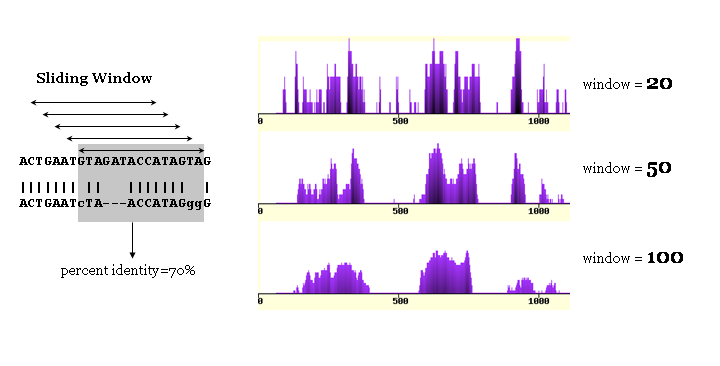
Sliding window size defines the smoothness of the conservation graph.
Larger values produce smoother graphs, while tend to result in loss of information content.
We find the optimum window size to be from 50 to 100 base pairs (bps).
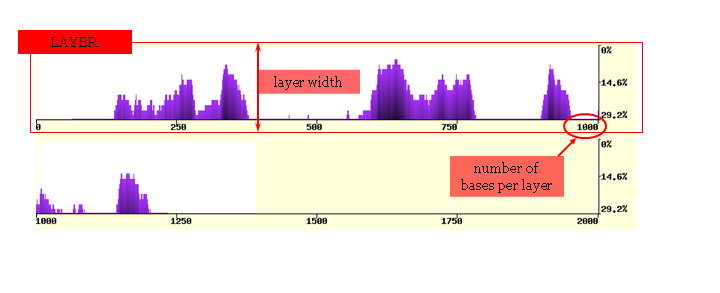
The conservation plot is presented as a series of horizontal layers. The number of bases per layer can
be varied to zoom in and out of the graphical display and vary the resolution of the alignment. The vertical width of each layer (layer width)
can also be adjusted to produce images of different sizes. The graphical display can be visualized using any
input sequence as the reference sequence, and this is achieved by changing the base organism preferences.
|
|
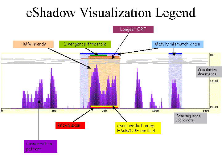
| 2. Mapping Conserved Regions |
| |
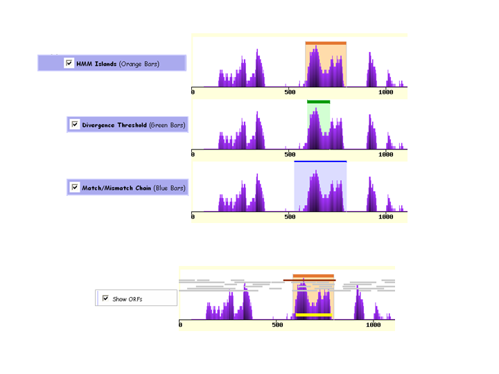
eShadow implements two different mathematical approaches for the identification of evolutionarily conserved
elements - HMM Islands and Divergence threshold. Conserved elements
identified by each approach are displayed in different colored graphs. All ORFs (Open Reading Frames) longer than 60 bps are detected
using stop codons present in all the species used to generate the alignment while each sequence is translated in all 6 different frames.
ORFs in different frames are plotted as 6 different rows of gray bars. The longest ORF for a putative exon is colored in dark red
(positive strand) or dark blue (negative strand) depending whether it was the forward or reverse direction. Boundaries of putative exons
(yellow bars on the plot) are defined using a set of fully conserved AG-GT splice sites.
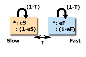
For the HMM Islands approach, there are three probabilities used to compute and detect conserved elements: eS and eF and T. eS and eF represent complete match emission probabilities while being in slow- or fast-mutation state, respectively. T is a transition probability from one state to another.
|
|
| 3. Features Annotation |
| |
DNA annotation information can be provided by the user using the Features annotation input option, and will be depicted as
red bars at the base of each layer of the conservation plot. Besides orienting the user within the contiguous stretch of DNA, these
features will also be used to guide the parameter optimization module in the HMM Islands approach. Often a DNA feature
can be an exon in nucleotide alignments or a domain in protein alignments. Please note that features annotation is species
dependant and therefore should be changed as the basis organism is varied. The location of each DNA feature should be
documented by individual line inputs. Every input should be denoted by two numbers: the starting and the ending numerical position
in the linear DNA separated by a space. For example, features annotation of two exons spanning intervals [50,100] and [200,250]
will have the following format:
50 100
200 250
|
|
| 4. Output Data |
| |
The eShadow tool provides the user with a default set of data files: (1) the input sequences, (2) ClustalW alignment and (3) output file
and (4) a .dnd file with evolutionary tree parameters (which could be used to plot a tree using tools such as the
Phylodendron). An extended output option is accessible
through the "Show eShadow text output below" option. The additional output files provide detailed statistics
of input sequences and the generated alignments including relative mismatch counts, substitution rates and information content analysis
when each additional species is being introduced into the alignment. Finally, it gives the coordinates of each identified conserved element
for the base sequence augmented by the scores and reading direction for each ORF
|
|
| 5. Plot Legend |
| |
|
